Creating new environment parameters
Reference grid
A reference grid is a case file in matlab format defining a grid (or more precisally, a photo of a grid, with instant injections). This file will be read by the simulator to load the electrical parameters of the grid, including for instance reactances and susceptances of lines, or the substations of which the grid productions are wired.
Currently, the simulator expects a IEEE-format case file for the reference_grid. .. Hint:: Such files can be found on the Matpower official repository. You can also find some details about the value of the matrices and columns of the IEEE format here.
The simulator cannot work with such a grid without some modifications, including the addition of artificial buses that will emulate the sister nodes of the original substations of the grid (two sister nodes per substation), and renaming and sorting the buses original ids. The build_new_parameters_environment script already performs this operation from the prompted filepath of the reference grid.
In a given environment, you might want to modify only the reference grid (for example, specifiying a different topological configuration) without modifying the other resources (reward_signal.py, chronics etc). In that case, you can run the following script, which will produce a valid reference grid for pypownet:
python -m parameters.make_reference_grid CASE_FILE_FILEPATH
where CASE_FILE_FILEPATH is the path to a grid case file (e.g. case30.m).
Chronics
In pratice, given injections and a grid topology, the flows within the grid will converge to a steady-steate, where electricity is carried from producers (e.g. nuclear central) toward consumers (e.g. a city). In real condition, the amount of demand cannot be controled: in other words, the injections relative to the loads are external to the operation of grid conduct. Besides, for several countries, the company responsible for natiowide grid conduct is different than the one responsible for the nationwide electricity production: in other words, the values of the productions are not in control of tehe grid conduct operators (they are by some other company, which also ensures that there is enough production to satisfy all demand). Those two macro aspects underlines that injections are effectively an input of the grid system in the context of grid conduct of natiowide scale.
For reproducibility purposes, productions and loads injections are thus an entry of the system (and not generated on the fly by the software), which can be controlled by a meta-user creating new chronics sets. An advantage to this approach is that the meta-user can control the timestep of the simulation: chronics entirely define the behavior of the flows within a grid. If the values of injections of a chronic have been generated with a timestep of 2 minutes, then the software will naturally be discretized into 2 minutes timesteps.
Chronics define the precise values of the entries of the Environment in which the grid will be subjected to through time. A game level folder contains one chronics folder, which contains one or several folders, which are the chronic folders (in the previous image, those chronic folders are named a, b, and c). More precisally, a chronic folder is made of 13 CSV files containing the temporal data for all the entries of the simulated grid system which are grouped into categories:
- grid injections (productions and consumptions temporal nominal values)
- grid previsions of injections which are given to the agents
- maintenance planned operations and grid external line breaking events (e.g. thunder breaking a line)
- simulation datetime and absolute IDs
- power lines nominal thermal limit for the whole chronic
Important
The delimiter in CSV files is always ‘;’
For visual purposes, here is a list of the files names in a chronic:
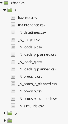
Important
The software will seek files with the exact filenames indicating in the above figure; your chronics should eventually contain 13 CSV files with the same name as listed above.
1. Grid injections
The grid injections (also called realized injections, since the values will effectively be an unmodified input of the grid) refer to four values:
- the active power (P) of productions
- the voltage magnitude (V) of productions
- the active power (P) of consumptions
- the reactive power (Q) of consumptions
Hint
In short, injections are the P and V values of productions, and P and Q values of loads, hence the respective names PV buses and PQ buses
The respective names of the associated chronic files are:
- _N_prods_p.csv
- _N_prods_v.csv
- _N_loads_p.csv
- _N_loads_q.csv
Each of these CSV files should have a header (which is not used in practice but mandatory) line of the desired number of file columns, followed by lines of ‘;’-separated values. Each line will correspond to one timestep, such that consecutive lines represent the injections of consecutive timesteps. The columns define the nominal values for each elements. For instance, if the grid is made of 5 productions and 8 loads, then both _N_prods_p.csv and _N_prods_v.csv should be made of 5 columns (so 4 ‘;’ per line), and both _N_loads_p.csv and _N_loads_q.csv should be made of 8 columns.
In practice, all of the active power values of productions are non-negative, because productions do produce active power. Sometimes, productions undergo some maintenance process (e.g. cleaning or repairing). This aspect can be controlled within the voltage magnitudes of productions (file _N_prods_v.csv), by setting the associated active production value to 0 (a production producing 0 effectively does not produce any electricity), or by setting the nominal value of the production to <= 0. Usually, productions voltage magnitudes are close to 1 (ranging from 0.94 to 1.06) in per-unit (understand: in the chronic file of production voltages). Any excessive value will almost automatically lead to a game over situation caused by a non-converging loadflow.
For the loads injections, the active power (_N_loads_p.csv) need to be non-negative (they represent the amount of demand of active power). The reactive power injections of the loads (_N_loads_q.csv) have no restrictions, but they usually are of lower magnitudes than the active values overall.
At initialization, the software will read the 4 realized files of the chronic. The first header row is discarded for each file, then the content is split into n lines, where n is the number of timesteps. At each timestep, the software will read the same line number in each of the 4 files, and insert the values into the grid. That is, the productions P and V values are replaces by the ones in the file, same for the loads P and Q values.
Note
If there are not enough active power production to satisfy all the active power demand, the slack bus will augment its output consequently, thus producing border effects on its adjacent lines. A good reflex is to ensure that the produced chronics has enough active power production to satisfy the active power demand at each timestep.
For illustration, suppose a grid is made of 2 productions and 2 consumptions, with the following realized injections which correspond to 3 timesteps (because there are 3 lines of data):
1 2 3 4 | prod0;prod1
10;5
11;6
12;6.4
|
1 2 3 4 | prod0;prod1
1;1
1;1
1;1
|
1 2 3 4 | load0;load1
7;8
9;8.4
11;7
|
1 2 3 4 | load0;load1
-2;3
-2;4
0;-1
|
For the first timestep, the software will read the highlighted line of each files (line 2 here, because this is the first timestep) and change the corresponding P, Q, V values of productions and loads.
2. Grid previsions of injections
Throughout the year, nationwide grid operators have constructed tools to estimate the future demands at various scales. This can be done because the consumptions pattern are very cyclical at many scales: day-to-day, week-to-week, year-to-year etc. For instance in France, on weekdays there is a peak of consumption at 7PM (probably when people get home and start cooking), while demand is relatively low during the night. Also, there is less demand during weekends, since a lot of companies work on weekdays (industries and companies are major electricity consumers). In that context, the simulator can give to the agents some predictions about the next timesteps injections (next loads PQ values come from demand estimation, and next prods PV values come from the schedules plans of producers). At each timestep, the agent will have access to both the current timestep injections, and the previsions (which are pre-simulation computed) for the next timestep.
The value of the previsions of injections (also called planned injections) are nominal for each production and each consumption (i.e. there are previsions for each injection gate). Consequently, the overall structure of the planned injections files are the same than the grid injections files. At each timestep, the software will read the next line for all the 4 realized injections file, as well as the same line for all 4 planned injections files, which should be named similarly to the realized files:
- _N_prods_p_planned.csv
- _N_prods_v_planned.csv
- _N_loads_p_planned.csv
- _N_loads_q_planned.csv
For illustration, given the following pair of realized/planned active power of productions, for the second timestep, the software will read the 3rd line in both files, replace the current productions P output by the read values, and carry the previsions of P values in an Observation:
1 2 3 4 | prod0;prod1
10;5
11;6
12;6.4
|
1 2 3 | prod0;prod1
10.9;5.8
12.9;6.3
|
In this example, the predictions, given at the first timestep, of the next timestep active power of productions are 10.9MW and 5.8MW for resp. the first production and the second production (seen on line 2 of _N_prods_p_planned.csv). In reality, at the next (second) timestep, the active power of productions inserted into the grid system are resp. 11MW and 5MW (seen on line 3 of _N_prods_p.csv).
3. Maintenance and external hazards
In real conditions, the power lines need to be maintained to ensure they are secure and work as intended. Such operations, called maintenance, involve switching power lines off for several hours, which make them unusable to ensure the safe functioning of the grid. The cause of maintenance are diverse (e.g. line repainting), but they are all known in advance (because they are planned by the grid manager). For the same reproducibility purposes as before, the maintenance are pre-computed prior to the simulation.
The file maintenance.csv provide all the maintenance that will happen during the chronic. Similarly to the previous files, the maintenance file has a header (not effectively use), followed by ‘;’-separated data e.g.:
1 2 3 4 5 | lines0;line1;line2;line3
1;0;0;0
0;0;0;0
0;2;0;3
0;0;0;0
|
The number of column of maintenance.csv should be equal to the number of power lines in the grid ( = the number of lines in the ‘branch’ matrix of the reference grid). Its number of lines should be the same as the files before, i.e. the number of timesteps of the chronic.
For a given timestep and a given power line (i.e. resp. a given line and a given column), a value d equal to 0 indicates that there are no maintenance starting at the corresponding timestep. A value d>0 indicates that a maintenance starts at this timestep, and that the power line will be unavailable (to be switched ON) for d timesteps starting from the current timestep.
Regarding maintenance, since in real life condition they are typically known, an Observation will also contain the previsions of the maintenance: given an horizon parameter (see later), the vecteur will contain one integer value for each power line, with a 0 value indicated no planned maintenance within the next horizon timestep, and a non-0 value indicating the number of timesteps before the next seen maintenance.
On top of maintenance operations, power grids are naturally subjected to external events that break lines from time to time. Such events could be related to nature (thunder hitting a power line, tree falling on some power line, etc), or could come from hardware malfunctioning. Such hazards are an entry of the system, and should be within the hazards.csv file which works exactly like the maintenance file, except that hazards are unpreditable in real life so no information is given to agents regarding forthcoming hazards.
4. Datetimes and IDs
The datetime file, _N_datetimes.csv contains the date associated with each timestep. As such, there is one date per line. The date should have the following format: ‘yyyy-mmm-dd;h:mm’ with ‘yyyy’ the 4 digits of the year, ‘mmm’ the 3 first letters in lowercase of the month, ‘dd’ the 1 or 2 digits of the day in the month, ‘h’ for the 1 or 2 digits of hour (from 0 to 23) and ‘mm’ for the 2 digits of minutes. Example of datetimes file:
1 2 3 4 5 | date;time
2018-jan-31;8:00
2018-jan-31;9:00
2018-jan-31;10:00
2018-jan-31;11:00
|
The datetimes entirely controls the timestep used for the simulation (this is due because the game mechanism is independent of time, so essentially the chronics dictatet the speed of temporal dimension). In the latter example, the duration between two timesteps is 1 hour, so an agent can only perform one action per hour. Because of regex limitations, the system cannot be discretized into seconds timesteps; you can create an issue on the official repository if you need such a feature.
The file _N_simu_ids.csv allows to bring consistency with the indexing of timesteps. This simple csv file has one column, one header line and one int or float value per timestep e.g.:
1 2 3 4 | id
0
1
2
|
With both examples, the timestep of id 2 happens at precisely 31st January of 2018 at 11AM.
5. Thermal limits
Finally, the last file of a chronic is the file _N_imaps.csv containing the nominal thermal limits of the power line: one thermal limit per line. The file consists in two lines: one is the header, not used (but should respect the correct number of columns), the other contain a list of ‘;’-separated float or int, indicating the thermal limits of each line e.g.:
1 2 | line0;line1;line2;line3
30;90;100;50
|
Note
There is one thermal limits per chronic, and not per game level, because chronics could be splitted by month, and thermal limits are technically lower during summer (higher heat), which could be emulated with lower thermal limits for the summer chronics.
Configuration file
The configuration file contains parameters that control the inner game mechanism in several ways. More precisally, the configuration file should be named configuration.yaml and should be placed at the top level of the considered level folder. As its name indicates, its format should be YAML, which is preferred here over JSON because of its possibility of comments and efficiency.
Hint
The template-building script build_new_parameters_environment.py automatically constructs such a file, with all the mandatory parameters, with default values.
Here is the list of (mandatory) parameters:
| loadflow_backend: | |
|---|---|
| backend used by the simulator to compute loadflows; can be “pypower” or “matpower” | |
| loadflow_mode: | model of loadflow used by the backend to compute loadflow; can be “AC” (alternative current) or “DC” (direct current) |
| max_seconds_per_timestep: | |
| not supported yet; maximum number of seconds allowed for the agent to produce an action at each timestep, before timeout | |
| hard_overflow_coefficient: | |
| percentage of thermal limit above which its current ampere value will make a line in hard-overflow (hard-overflowed lines break instantly) | |
| n_timesteps_hard_overflow_is_broken: | |
| duration in timesteps a hard-overflowed line is broken: the line needs repairs and cannot be switched ON for this number of timesteps | |
| n_timesteps_consecutive_soft_overflow_breaks: | |
| number of consecutive timesteps at the end of which an overflowed (but not hard-overflowed) line is breaks (heat build-up) | |
| n_timesteps_soft_overflow_is_broken: | |
| duration in timesteps a soft-overflowed line is broken: the line needs repairs and cannot be switched ON for this number of timesteps | |
| n_timesteps_horizon_maintenance: | |
| number of future timesteps for which previsions of maintenance are provided in an Observation | |
| max_number_prods_game_over: | |
| maximum (inclusive) number of isolated productions tolerated before a game over signal is raised | |
| max_number_loads_game_over: | |
| maximum (inclusive) number of isolated consumptions tolerated before a game over signal is raised | |
| n_timesteps_actionned_line_reactionable: | |
| cooldown in timesteps on the activations of lines: number of timesteps to wait before a controler-activated line (switched ON or OFF) can be activated again by the controler | |
| n_timesteps_actionned_node_reactionable: | |
| cooldown in timesteps on the activations of substations: number of timesteps to wait before a controler-activated substation (any node-splitting operation) can be activated again by the controler | |
| n_timesteps_pending_line_reactionable_when_overflowed: | |
| not supported yet | |
| n_timesteps_pending_node_reactionable_when_overflowed: | |
| not supported yet | |
| max_number_actionned_substations: | |
| per timestep maximum (inclusive) number of separated controler-activated substations (ie with at least one node-splitting operation): an action with strictly more activated substations than this value is replaced by a do-nothing action | |
| max_number_actionned_lines: | |
| per timestep maximum (inclusive) number of separated controler-activated lines (ie switched ON or OFF): an action with strictly more activated lines than this value is replaced by a do-nothing action | |
| max_number_actionned_total: | |
| per timestep maximum (inclusive) number of separated controler-activated lines+substations: an action with strictly more activated lines+substations than this value is replaced by a do-nothing action | |
Here is the default configuration.yaml (produced by the template-creater script):
1 2 3 4 5 6 7 8 9 10 11 12 13 14 15 16 17 18 19 20 21 22 23 24 25 26 27 | loadflow_backend: pypower
#loadflow_backend: matpower
loadflow_mode: AC # alternative current: more precise model but longer to process
#loadflow_mode: DC # direct current: more simplist and faster model
max_seconds_per_timestep: 1.0 # time in seconds before player is timedout
hard_overflow_coefficient: 1.5 # % of line capacity usage above which a line will break bc of hard overflow
n_timesteps_hard_overflow_is_broken: 10 # number of timesteps a hard overflow broken line is broken
n_timesteps_consecutive_soft_overflow_breaks: 3 # number of consecutive timesteps for a line to be overflowed b4 break
n_timesteps_soft_overflow_is_broken: 5 # number of timesteps a soft overflow broken line is broken
n_timesteps_horizon_maintenance: 20 # number of immediate future timesteps for planned maintenance prevision
max_number_prods_game_over: 10 # number of tolerated isolated productions before game over
max_number_loads_game_over: 10 # number of tolerated isolated loads before game over
n_timesteps_actionned_line_reactionable: 3 # number of consecutive timesteps before a switched line can be switched again
n_timesteps_actionned_node_reactionable: 3 # number of consecutive timesteps before a topology-changed node can be changed again
n_timesteps_pending_line_reactionable_when_overflowed: 1 # number of cons. timesteps before a line waiting to be reactionable is reactionable if it is overflowed
n_timesteps_pending_node_reactionable_when_overflowed: 1 # number of cons. timesteps before a none waiting to be reactionable is reactionable if it has an overflowed line
max_number_actionned_substations: 7 # max number of changes tolerated in number of substations per timestep; actions with more than max_number_actionned_substations have at least one 1 value are replaced by do-nothing action
max_number_actionned_lines: 10 # max number of changes tolerated in number of lines per timestep; actions with more than max_number_actionned_lines are switched are replaced by do-nothing action
max_number_actionned_total: 15 # combination of 2 previous parameters; actions with more than max_number_total_actionned elements (substation or line) have a switch are replaced by do-nothing action
|
Reward signal file
The reward signal is the function that computes the reward which will be fed to the models at each timestep, after they perform an action given an observation. This is the typical reward function that feeds reinforcement learning models. pypownet is able to handle custom reward signals, as there is not yet particular reward functions that seem to drive the optimisation of useful dispatchers-like controlers. For a given environment, if not explicit reward signal is given, the simulator will use the default reward signal which always outputs 0: this implies no learning for models.
Formally, the reward signal should be a class CustomRewardSignal daughter class of RewardSignal (default reward signal), placed within each environment folder (e.g. in default14/).
The python file containing this class should be named reward_signal.py, otherwise it won’t be taken into account by the simulator.
Here is the default reward signal:
1 2 3 4 5 6 7 8 9 10 11 12 13 14 15 16 17 18 19 20 21 | class RewardSignal(object):
""" This is the basic template for the reward signal class that should at least implement a compute_reward
method with an observation of pypownet.environment.Observation, an action of pypownet.environment.Action and a flag
which is an exception of the environment package.
"""
def __init__(self):
pass
def compute_reward(self, observation, action, flag):
""" Effectively computes a reward given the current observation, the action taken (some actions are penalized)
as well as the flag reward, which contains information regarding the latter game step, including the game
over exceptions raised or illegal line reconnections.
:param observation: an instance of pypownet.environment.Observation
:param action: an instance of pypownet.game.Action
:param flag: an exception either of pypownet.environment.DivergingLoadflowException,
pypownet.environment.IllegalActionException, pypownet.environment.TooManyProductionsCut or
pypownet.environment.TooManyConsumptionsCut
:return: a list of subrewards as floats or int (potentially a list with only one value)
"""
return [0.]
|
CustomRewardSignal should at least implement a function CustomRewardSignal.compute_reward which takes as input:
- the current observation of the simulated grid system
- the last action played by the player (which lead to the above observation)
- the simulator flag, which is an instance of a customized Exception of pypownet indicating game over triggers if any (i.e. if the last action lead to a game over)
The current observation is an instance of pypownet.environment.Observation, see Reading observations for further information about observations. The last action is an instance of pypownet.game.Action. The simulator flag is either None if the last step did not lead to a game over. However, if the last step lead to a game over, the input flag will be of either type, representing various types of pypownet exceptions. flag will be an instance of either exceptions:
- pypownet.environment.DivergingLoadflowException: game over provocked by a non-converging grid; might happend when the grid is not connexe, or in too poor shape such that flows diverge
- pypownet.environment.TooManyProductionsCut: the number of isolated productions has exceeded the maximum number of tolerated isolated productions; see Configuration file
- pypownet.environment.TooManyConsumptionsCut: the number of isolated consumptions has exceeded the maximum number of tolerated isolated consumptions; see Configuration file
- pypownet.environment.IllegalActionException: at least one illegal action (such as reconnecting unavailable broken lines) has been performed
Among those exceptions, pypownet.environment.IllegalActionException is special: this is the only one which does not mean that there wxas a game over. Actually, if some lines status are attempted to be switched while the associated lines are broken, the simulator will simply change the action such that the switch is deactivated, without any cost; for practical justifications, we could imagine an automatous mechanism that checks whether a line is available before switching its status.
Here is a concrete example of a custom reward signal used in the environment default14/ (for more insight about this class, see Default environments):
1 2 3 4 5 6 7 8 9 10 11 12 13 14 15 16 17 18 19 20 21 22 23 24 25 26 27 28 29 30 31 32 33 34 35 36 37 38 39 40 41 42 43 44 45 46 47 48 49 50 51 52 53 54 55 56 57 58 59 60 61 62 63 64 65 66 67 68 69 70 71 72 73 74 75 76 77 78 79 80 81 82 83 84 85 86 87 88 89 90 91 92 93 94 95 96 97 98 99 100 101 102 103 104 105 106 107 108 109 110 111 112 113 114 115 116 117 118 119 120 121 122 123 124 125 126 127 128 129 130 131 | import pypownet.environment
import pypownet.reward_signal
import numpy as np
class CustomRewardSignal(pypownet.reward_signal.RewardSignal):
def __init__(self):
super().__init__()
constant = 14
# Hyper-parameters for the subrewards
# Mult factor for line capacity usage subreward
self.multiplicative_factor_line_usage_reward = -1.
# Multiplicative factor for total number of differed nodes in the grid and reference grid
self.multiplicative_factor_distance_initial_grid = -.02
# Multiplicative factor total number of isolated prods and loads in the grid
self.multiplicative_factor_number_loads_cut = -constant / 5.
self.multiplicative_factor_number_prods_cut = -constant / 10.
# Reward when the grid is not connexe (at least two islands)
self.connexity_exception_reward = -constant
# Reward in case of loadflow software error (e.g. 0 line ON)
self.loadflow_exception_reward = -constant
# Multiplicative factor for the total number of illegal lines reconnections
self.multiplicative_factor_number_illegal_lines_reconnection = -constant / 100.
# Reward when the maximum number of isolated loads or prods are exceeded
self.too_many_productions_cut = -constant
self.too_many_consumptions_cut = -constant
# Action cost reward hyperparameters
self.multiplicative_factor_number_line_switches = -.2 # equivalent to - cost of line switch
self.multiplicative_factor_number_node_switches = -.1 # equivalent to - cost of node switch
def compute_reward(self, observation, action, flag):
# First, check for flag raised during step, as they indicate errors from grid computations (usually game over)
if flag is not None:
if isinstance(flag, pypownet.environment.DivergingLoadflowException):
reward_aslist = [0., 0., -self.__get_action_cost(action), self.loadflow_exception_reward, 0.]
elif isinstance(flag, pypownet.environment.IllegalActionException):
# If some broken lines are attempted to be switched on, put the switches to 0, and add penalty to
# the reward consequent to the newly submitted action
reward_aslist = self.compute_reward(observation, action, flag=None)
n_illegal_reconnections = np.sum(flag.illegal_lines_reconnections)
illegal_reconnections_subreward = self.multiplicative_factor_number_illegal_lines_reconnection * \
n_illegal_reconnections
reward_aslist[2] += illegal_reconnections_subreward
elif isinstance(flag, pypownet.environment.TooManyProductionsCut):
reward_aslist = [0., self.too_many_productions_cut, 0., 0., 0.]
elif isinstance(flag, pypownet.environment.TooManyConsumptionsCut):
reward_aslist = [self.too_many_consumptions_cut, 0., 0., 0., 0.]
else: # Should not happen
raise flag
else:
# Load cut reward
number_cut_loads = sum(observation.are_loads_cut)
load_cut_reward = self.multiplicative_factor_number_loads_cut * number_cut_loads
# Prod cut reward
number_cut_prods = sum(observation.are_productions_cut)
prod_cut_reward = self.multiplicative_factor_number_prods_cut * number_cut_prods
# Reference grid distance reward
reference_grid_distance = self.__get_distance_reference_grid(observation)
reference_grid_distance_reward = self.multiplicative_factor_distance_initial_grid * reference_grid_distance
# Action cost reward: compute the number of line switches, node switches, and return the associated reward
action_cost_reward = -self.__get_action_cost(action)
# The line usage subreward is the sum of the square of the lines capacity usage
lines_capacity_usage = self.__get_lines_capacity_usage(observation)
line_usage_reward = self.multiplicative_factor_line_usage_reward * np.sum(np.square(lines_capacity_usage))
# Format reward
reward_aslist = [load_cut_reward, prod_cut_reward, action_cost_reward, reference_grid_distance_reward,
line_usage_reward]
return reward_aslist
def __get_action_cost(self, action):
# Action cost reward: compute the number of line switches, node switches, and return the associated reward
""" Compute the >=0 cost of an action. We define the cost of an action as the sum of the cost of node-splitting
and the cost of lines status switches. In short, the function sums the number of 1 in the action vector, since
they represent activation of switches. The two parameters self.cost_node_switch and self.cost_line_switch
control resp the cost of 1 node switch activation and 1 line status switch activation.
:param action: an instance of Action or a binary numpy array of length self.action_space.n
:return: a >=0 float of the cost of the action
"""
# Computes the number of activated switches of the action
number_line_switches = np.sum(action.get_lines_status_subaction())
number_prod_nodes_switches = np.sum(action.get_prods_switches_subaction())
number_load_nodes_switches = np.sum(action.get_loads_switches_subaction())
number_line_or_nodes_switches = np.sum(action.get_lines_or_switches_subaction())
number_line_ex_nodes_switches = np.sum(action.get_lines_ex_switches_subaction())
number_node_switches = number_prod_nodes_switches + number_load_nodes_switches + \
number_line_or_nodes_switches + number_line_ex_nodes_switches
action_cost = self.multiplicative_factor_number_node_switches * number_node_switches + \
self.multiplicative_factor_number_line_switches * number_line_switches
return action_cost
@staticmethod
def __get_lines_capacity_usage(observation):
ampere_flows = observation.ampere_flows
thermal_limits = observation.thermal_limits
lines_capacity_usage = np.divide(ampere_flows, thermal_limits)
return lines_capacity_usage
@staticmethod
def __get_distance_reference_grid(observation):
# Reference grid distance reward
""" Computes the distance of the current observation with the reference grid (i.e. initial grid of the game).
The distance is computed as the number of different nodes on which two identical elements are wired. For
instance, if the production of first current substation is wired on the node 1, and the one of the first initial
substation is wired on the node 0, then their is a distance of 1 (there are different) between the current and
reference grid (for this production). The total distance is the sum of those values (0 or 1) for all the
elements of the grid (productions, loads, origin of lines, extremity of lines).
:return: the number of different nodes between the current topology and the initial one
"""
#initial_topology = np.asarray(self.game.get_initial_topology())
initial_topology = np.concatenate((observation.initial_productions_nodes, observation.initial_loads_nodes,
observation.initial_lines_or_nodes, observation.initial_lines_ex_nodes))
current_topology = np.concatenate((observation.productions_nodes, observation.loads_nodes,
observation.lines_or_nodes, observation.lines_ex_nodes))
return np.sum((initial_topology != current_topology)) # Sum of nodes that are different
|